Light pollution is measured with Sky Quality Meters, calibrated cameras, and satellites — each capturing a different slice of the same problem. LoNNe’s four field intercomparison campaigns, run across Europe between 2013 and 2016, proved that no single instrument tells the whole story, and that instruments from the same model line can disagree by up to 0.2 magnitudes under identical conditions. Kyba et al. (2017, Science Advances) showed the lit surface area of Earth is growing at 2.2% per year — a figure most sources cite without explaining that it was measured by a satellite blind to the blue wavelengths now dominating street lighting. For the foundational science behind what light pollution is and why it matters, see our overview of light pollution: science, ecology, and solutions. This article is for researchers, dark-sky practitioners, and citizen scientists who want to move past the number and understand the methodology behind it.
The Bortle Scale Explained
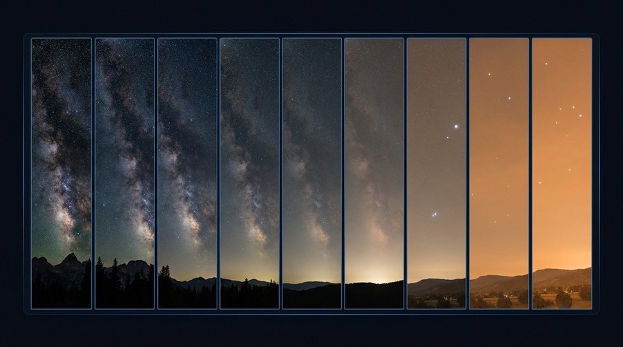
Nine numbered classes translate naked-eye sky observations into a single, portable quality score — no instrument required.

John E. Bortle published his scale in Sky & Telescope in February 2001 as a practical tool for amateur astronomers frustrated by the lack of a common vocabulary for describing observing conditions. The problem was real. One observer’s “clear rural sky” was another’s “suburban muddle” — there was no shared reference point. Bortle’s nine classes, anchored to specific celestial objects visible to the naked eye, gave observers a common language. Class 1 represents the darkest accessible skies on Earth; Class 9 is the inner-city sky where only the Moon and a handful of bright planets remain.
The scale maps reasonably well onto Sky Quality Meter readings, though the correspondence is statistical rather than exact. The table below shows representative values for all nine classes, with naked-eye limiting magnitude (NELM) and SQM equivalents:
| Bortle Class | Label | NELM | SQM (mag/arcsec²) | Visibility landmarks |
|---|---|---|---|---|
| 1 | Excellent dark sky | 7.6–8.0 | 21.9–22.0+ | Zodiacal light, gegenschein, Milky Way casts shadows |
| 2 | Truly dark sky | 7.1–7.5 | 21.5–21.9 | M33 direct, air glow on horizon visible |
| 3 | Rural sky | 6.6–7.0 | 21.3–21.5 | Milky Way finely structured, zodiacal band faint |
| 4 | Rural/suburban transition | 6.1–6.5 | 20.4–21.3 | M33 with averted vision, slight glow at horizon |
| 5 | Suburban sky | 5.6–6.0 | 19.9–20.4 | Milky Way washed out at zenith, orange glow visible |
| 6 | Bright suburban sky | 5.1–5.5 | 18.9–19.9 | Only central Milky Way at zenith, extensive glow |
| 7 | Suburban/urban transition | 4.6–5.0 | 18.0–18.9 | Milky Way invisible, sky grey-white at zenith |
| 8 | City sky | 4.1–4.5 | 18.0–18.5 | Only obvious star patterns visible, orange-white sky |
| 9 | Inner-city sky | ≤4.0 | ≤18.0 | Useless for most observing, only Moon and bright planets |
NELM is where the scale becomes tricky. Two experienced observers at the same site on the same night routinely differ by 0.5 magnitudes in their limiting magnitude estimates — equivalent to a full Bortle class difference. Age, dark adaptation, averted vision technique, and individual retinal sensitivity all contribute. A 2014 review of the Class 4 benchmark — M33 visible with averted vision — found the criterion observer-dependent enough to create systematic classification errors of one class in either direction. Bortle’s scale is an excellent communication tool and a useful field reference. It is not a calibration standard. For sites where Bortle values are published alongside measured sky-quality readings, see our article on dark sky places in Europe.
The SQM removes observer subjectivity. It measures the zenith sky in under three seconds, reports in mag/arcsec², and can be logged automatically. The Bortle–SQM correspondence shown in the table gives practitioners a translation tool, but the numbers are median values from field data rather than theoretical derivations. A Class 4 sky might read anywhere from 20.1 to 21.5 mag/arcsec² depending on atmospheric conditions, moon phase, and seasonal airglow variation. The scale is a proxy. A good proxy — but not a measurement.
The Sky Quality Meter (SQM) — Your Primary Instrument
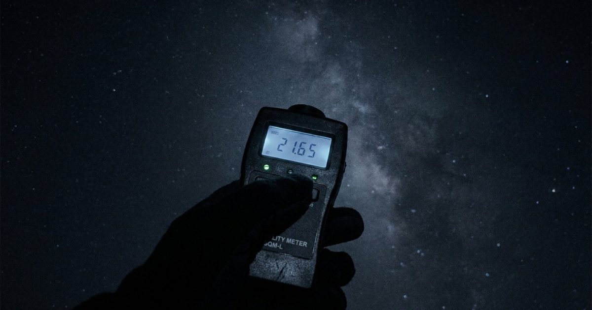
The SQM is a single-band silicon photodetector that converts zenith sky brightness into mag/arcsec² in under three seconds.
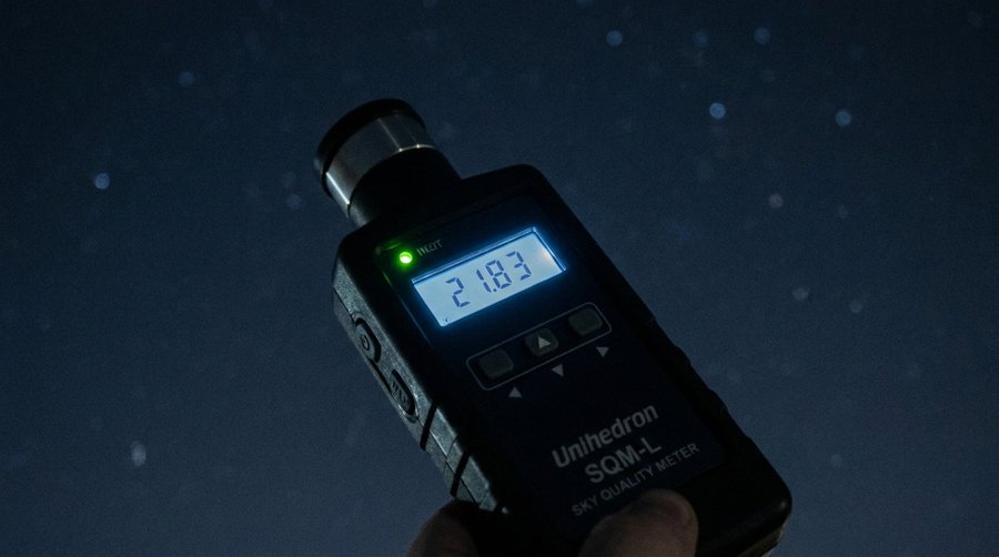
The Sky Quality Meter, manufactured by Unihedron in Ontario, Canada, became the de facto field standard for light pollution research for straightforward reasons: it is robust, affordable (around EUR 100–150 depending on variant), simple to operate, and consistent enough for inter-site comparisons when used with proper protocol. The device contains a silicon photodetector behind a narrowband interference filter centred at approximately 550 nm. It samples the zenith sky, converts the photon flux to an astronomical magnitude scale, and displays the result in mag/arcsec². Higher numbers mean darker skies. A reading of 22.0 is pristine; 20.0 is rural with a visible glow; below 18.0 is urban.
SQM Variants: Which Device for Which Purpose
Unihedron produces three main variants, and choosing the wrong one creates systematic errors that invalidate longitudinal comparisons.
The SQM-L is the narrow-field version. Its lens limits the effective field of view to approximately 20° full-width at half maximum (FWHM). This is the instrument LoNNe intercomparison campaigns standardised on for research-grade measurements — the narrow cone reduces contamination from horizon glow, artificial sources in the lateral sky, and atmospheric variations at low elevation angles. Point it straight up and you get a clean zenith reading.
The SQM-LU adds USB connectivity via the same optical assembly as the SQM-L — FWHM remains approximately 20°. The USB connection enables direct data logging and real-time computer readout, making the LU suitable for automated monitoring setups where data are streamed continuously. The original SQM (without the “L” suffix) uses a wider acceptance angle with approximately 42° half-width at half maximum — it samples a much larger portion of the hemisphere and is more susceptible to horizon contamination. Researchers comparing data from SQM (original) and SQM-L units should not treat the readings as interchangeable.
The SQM-LU-DL adds onboard data logging to the LU optical assembly. It is the preferred instrument for autonomous long-term monitoring — no laptop required, measurements stored to internal memory and downloadable periodically. LoNNe recommended the LU-DL for unmanned multi-night campaigns precisely because it removes the observer-presence variable. An observer breathing or moving near the instrument creates stray heat and micro-vibration; an unattended unit in a fixed mount does not. For a detailed comparison of variants, applications, and purchasing criteria, see our SQM buyer’s guide: L vs. LU vs. LU-DL.
Two Systematic Limitations You Need to Know
The SQM has two limitations that matter practically — and which no published monitoring protocol should omit.
Zenith bias. The instrument points straight up by design. In suburban environments, the brightest source of sky glow often comes not from directly overhead but from the near-horizon dome — city lights on the skyline scatter light at low elevation angles that an SQM never sees. A site with moderate zenith readings may be far worse for an astronomer working at 30° elevation. The difference can reach 0.5 mag/arcsec² between the zenith and a low-elevation pointing — an error that matters when you are trying to compare a site’s overall usability for visual or photographic observing against its reported SQM value.
The LED blindspot. The SQM filter is centred on the visual band — calibrated in an era when sodium-vapour lamps dominated street lighting. High-pressure sodium (HPS) lamps peak at around 589 nm: comfortably within the SQM’s passband. White LED street lights are different. Their spectral output includes a substantial blue component in the 400–505 nm range — the broad peak of the blue LED pump beneath the phosphor conversion layer. The SQM filter suppresses sensitivity at these wavelengths. The practical consequence: as cities replace HPS lamps with white LEDs, the SQM underreports the change in sky brightness. It cannot see the blue light that LEDs are adding. Hänel et al. (2018, Journal of Quantitative Spectroscopy and Radiative Transfer, 205: 278–290) quantified this systematic underreporting using calibrated fisheye cameras with colour channels — the same cameras that can separate the blue contribution from the broadband reading. An SQM at an LED-retrofitted suburban site is measuring the sky with an instrument that cannot fully see what has changed. This is not a device flaw. It is a calibration-era mismatch, and it is why LoNNe’s intercomparison campaigns insisted on multi-instrument setups at every site.
Advanced Methods: Beyond the SQM
When a single zenith reading is not enough, calibrated all-sky cameras capture the full hemisphere — and the full spectral problem.
Hänel et al. 2018 benchmarked five instrument classes at the same field sites during LoNNe-affiliated campaigns: hand-held SQM, SQM-L on fixed mount, all-sky fisheye DSLR camera, calibrated luminance meter, and dedicated all-sky photometer. Their conclusion was clear: calibrated consumer digital cameras with fisheye lenses provide the best balance between ease of use and richness of obtainable information. A single 180° fisheye exposure, taken with a camera whose spectral response curve is characterised and whose flat-field calibration is applied, yields sky brightness across the full hemisphere in three colour channels within approximately five minutes of post-processing. The arXiv preprint that preceded the paper (arXiv:1709.09558) gave the methods community early access and has been widely cited as the methodological reference for European field campaigns since 2018.
Three additional methods complete the toolkit. Calibrated luminance meters and spectroradiometers provide point measurements with spectral resolution — they can separate sodium and LED contributions wavelength by wavelength, which no broadband instrument can do. LoNNe intercomparison campaigns included spectroradiometers at each site to give the field the spectral ground truth that SQMs cannot provide. Synthetic SQM is an NPS-developed technique that estimates sky brightness from fisheye images by convolving the image with the SQM angular response function — effectively extracting a simulated SQM reading from a photograph without the physical instrument present. Useful for reanalysing archival imagery. Extinction coefficient measurement — tracking standard stars at different airmass values to determine how much light the atmosphere absorbs per unit path length — gives the atmospheric transparency context that makes all other measurements interpretable. An extinction above 0.3 mag/airmass signals poor transparency from aerosols, humidity, or smoke; below 0.15 is considered photometric. Results from high-extinction nights cannot be compared directly to low-extinction nights without correction.
Reading the Numbers: Units and What They Mean
Two units describe the same sky — mag/arcsec² for astronomers, μcd/m² for lighting engineers. Neither converts intuitively to the other.
The magnitude system is ancient — it descends from Hipparchus — and it runs backwards. A larger number means a dimmer sky. The scale is logarithmic: a difference of 5 magnitudes corresponds to a factor of exactly 100 in brightness. A sky at 22.0 mag/arcsec² is 100 times darker than a sky at 17.0 mag/arcsec². Each single magnitude step is a factor of 2.512 (the fifth root of 100). This trips up practitioners coming from the engineering side, where “larger number = brighter” is the intuitive expectation.
Lighting engineers and public health researchers use μcd/m² — microcandela per square metre — a linear unit where larger equals brighter. The two communities rarely share data directly, because the conversion is non-linear and the reference point definitions differ slightly by source. The table below gives five reference values calibrated against the Garstang (1986) model and the Falchi et al. (2016) atlas calibration:
| Sky condition | mag/arcsec² | μcd/m² | Bortle class (approx.) |
|---|---|---|---|
| Pristine dark (natural reference) | 22.0 | 172 | 1 |
| Truly dark rural | 21.5 | 274 | 2 |
| Rural with glow | 20.5 | 686 | 4–5 |
| Bright suburban | 19.0 | 2,728 | 7 |
| Urban core | 17.5 | 10,867 | 8–9 |
The natural sky background — the “pristine” reference — is not zero. It includes airglow (oxygen emission at 557.7 nm and 630 nm, sodium emission at 589 nm from the mesosphere), integrated starlight, zodiacal light, and the cosmic background. The CIE and IDA use approximately 174 μcd/m² as the natural zenithal sky brightness reference; Garstang’s model gives 172 μcd/m² — close enough that the difference is within observational error for ground-based instruments.
The Light Pollution Ratio (LPR), also called the artificial-to-natural luminance ratio (ALR), expresses sky brightness as a multiple of the natural background. LPR = 0 means no artificial contribution. LPR < 0.3 means the sky is excellent — natural darkness well preserved. LPR > 2.0 means the natural sky background is no longer perceptible to the naked eye; the artificial component dominates completely. Most of European low-density rural landscape sits between 0.3 and 1.0. Major cities exceed 10.
Walker’s Law gives a first-order prediction of sky brightness contribution from a city: b = C × P × d^(−2.5), where b is sky brightness in nanoLamberts, P is city population, d is distance in appropriate units, and C is an empirical constant derived from observations (Walker 1977, Publications of the Astronomical Society of the Pacific, 89: 405–409). The exponent −2.5 is the departure from pure inverse-square (which would give −2.0). The difference matters: at −2.5, doubling your distance from a city reduces sky brightness by a factor of about 5.7 rather than the factor of 4 you would expect from simple geometry. The additional steepening comes from atmospheric forward scattering — light from near-horizon sources follows a longer path through the atmosphere and gets absorbed and scattered more efficiently than the geometry alone would predict. Walker’s Law holds reasonably well up to 50–100 km; beyond that, terrain masking and Earth’s curvature cause faster falloff than the model predicts.
Global Data: What Satellites Tell Us — and What They Miss
VIIRS detects lit surface area from 500 km altitude — but its spectral window stops exactly where LED emissions begin.
The VIIRS Day/Night Band (DNB) aboard Suomi-NPP (launched 2011) and NOAA-20 (launched 2017) is the primary instrument for global light pollution mapping from space. Spatial resolution is approximately 750 m at nadir — far coarser than the SQM ground point, but global in coverage. The DNB spectral window runs from 505 to 890 nm. That lower bound is not arbitrary: it is the engineering result of suppressing solar contamination at wavelengths below ~500 nm. It is also the exact spectral boundary where modern white LED street lighting does a large fraction of its work.
White LED lamps used in street lighting consist of a blue LED pump at 440–480 nm exciting a broad-spectrum phosphor. The output includes a distinct blue peak below 505 nm that VIIRS cannot detect. Every LED-retrofitted city in Europe is emitting light that the satellite that is supposed to track global light pollution cannot see. The gap is not a satellite malfunction. It is an instrument-design consequence that interacts badly with a technology transition the instrument was not designed to track.
The Kyba 2017 finding requires two clarifications. Kyba et al. (2017, Science Advances) used VIIRS DNB data from 2012 to 2016 and found that Earth’s lit surface area was growing at 2.2% per year globally, while total radiance was growing at 1.8% per year. These are different quantities. Lit surface area growth means the illuminated footprint is expanding — more roads, more car parks, more formerly unlit peri-urban areas brought into the lit network. Radiance growth at 1.8% measures how much brighter existing lit areas are becoming. Both are VIIRS measurements and both carry the same LED-blindspot caveat: they measure only what is detectable above 505 nm. The 2.2% lit-surface figure is a floor estimate. Real growth in human-visible and ecologically relevant light is higher, because the blue component of LED light that VIIRS cannot see is being added to every retrofitted city at exactly the moment when the satellite is declared to be tracking the problem.
Kyba et al. (2023, Science 379: 265–268) confirmed this interpretation with an independent method. Citizen scientists in Globe at Night reported stellar visibility changes from 51,351 observations at 19,262 locations across 2011–2022. Sky brightness derived from stellar visibility estimates increased at 9.6% per year — equivalent to doubling every eight years. This is the same sky, the same time period, the same phenomenon — but measured from the ground, by the human eye, which has no spectral blind spot in the blue. Satellite data showed a much smaller trend. Ground-based citizen science showed a much larger one. The divergence is the LED blindspot in quantitative form. For the full context on these two studies and their methodological differences, see our companion article on the Falchi 2016 and Kyba 2017 data explained.
Falchi et al. (2016, Science Advances) took a different approach. Rather than using satellite data alone, the World Atlas of Artificial Night Sky Brightness used VIIRS radiance data as input to an atmospheric radiative transfer model — calculating how satellite-detected radiance at altitude translates to artificial sky brightness at ground level, accounting for scattering through the full atmospheric column. Calibration against more than 35,000 ground-based SQM measurements provided the empirical anchoring. The results: 83% of the world’s population and 99% of Europeans and Americans live under light-polluted skies; 60% of Europeans cannot see the Milky Way from their homes. The atlas remains the primary global reference for artificial sky brightness, though its VIIRS input carries the same LED-blindspot limitation. For those wanting to reduce the light pollution behind these numbers, see our guide to light pollution solutions.
The LoNNe Intercomparison Campaigns
Four field campaigns across Europe, 2013–2016, tested whether SQMs, cameras, and luxmeters from different labs agree — and found they often do not.
Instrument intercomparison is the internal quality control of measurement science. Before trend data from different observatories can be combined into a single dataset, someone has to verify that the instruments agree — that a 21.0 reading on one SQM corresponds to the same physical sky brightness as a 21.0 reading on a different SQM, measured at a different site by a different observer. The assumption of interchangeability is so convenient that it often goes untested. LoNNe (COST Action ES1204) tested it.
Between 2013 and 2016, LoNNe coordinated a series of field intercomparison campaigns at European sites representing a range of sky conditions — from dark rural sites to urban environments. Instruments brought by multiple research groups to the same site on the same night. Results logged simultaneously. Discrepancies identified, characterised, and published. The campaign structure allowed systematic uncertainties — instrument-to-instrument offsets that persist regardless of conditions — to be separated from random measurement noise.
The documented locations and sequences are as follows:
| Campaign | Location | Year | Key instruments |
|---|---|---|---|
| 1 | Lastovo Island, Croatia | 2013 | Multiple SQMs, training school component, dark reference site |
| 2 | UCM campus, Madrid, Spain | 2014 | SQM-L array, fisheye DSLR, luxmeter, urban sky conditions |
| 3 | Torniella and Florence, Italy | 2015 | SQM variants, calibrated camera, spectroradiometer, rural-to-peri-urban gradient |
| 4 | Montsec Observatory, Spain | 2016 | Full instrument suite, dark site reference, STARS4ALL collaboration |
An additional intercomparison was organised at Chelmos, Greece, in September 2015 in conjunction with the LoNNe working group meeting in Athens — adding a fifth measurement event across the network period, though the four above constitute the primary campaign sequence documented in LoNNe outputs.
The findings from these campaigns are not encouraging for anyone who assumed that identical instruments give identical results. The overall measurement uncertainty for SQM instruments in field conditions — combining unit-to-unit variability, calibration drift, and protocol differences — was characterised at approximately ±0.19 mag/arcsec² for the SQM-L (Report of the 2014 LoNNe Intercomparison Campaign). That figure sounds small until you consider that the sky-brightness trends LoNNe researchers were trying to detect — the annual change in sky brightness from LED deployment, energy-saving measures, or regulatory interventions — operate at scales of 0.02 to 0.05 mag/arcsec² per year. An instrument uncertainty nearly four times larger than the annual trend is not a rounding error. It is the dominant source of noise in the measurement.
Three actionable conclusions emerged from the campaign series:
First, cross-calibration is mandatory before combining data from different observers or different SQM units. Two instruments of identical model number, purchased from the same batch, can differ systematically by enough to mask or mimic a year’s worth of sky-brightness change. Cross-calibration against a common reference site — ideally a photometrically stable dark site on a moonless, low-extinction night — is the minimum requirement for multi-observer data. LoNNe recommended running this calibration at the start of any multi-instrument campaign and repeating it at the end.
Second, all-sky fisheye cameras outperform single-pointing SQMs for characterising spatial sky-glow distribution. A fisheye image captures the full hemisphere simultaneously, allowing the sky glow gradient from different azimuth directions to be mapped, and enabling the extraction of a synthetic SQM value for any pointing direction — including comparisons across time that are more robust to variable atmospheric extinction. LoNNe recommended all-sky photometry as the gold standard for intercomparison events, with SQMs retained for long-term unattended monitoring where camera logistics are impractical.
Third, LED-transition sites require spectral instruments. A standard SQM at a site undergoing lamp replacement from HPS to LED may report little or no change in sky brightness — because the instrument cannot see the new blue emission the LEDs are contributing. A spectroradiometer or calibrated RGB camera at the same site will show a measurable spectral shift toward blue wavelengths even when the broadband SQM reading remains stable. The intercomparison campaigns that included spectroradiometers — particularly the Torniella and Montsec campaigns — demonstrated this mismatch directly, connecting LoNNe’s field hardware to the same LED-blindspot story that Kyba et al. 2017 documented from orbit. The connection between what the satellite missed and what the SQM missed is not coincidental. Both instruments were calibrated against a sodium-lamp world. Both are being asked to track a blue-LED world. No other source can report these findings from primary participation in LoNNe’s campaign series.
For the extended analysis of what these campaigns revealed about instrument protocol, calibration procedures, and measurement uncertainty — including the full discussion of fisheye camera calibration methodology — see our deep-dive article on the LoNNe intercomparison campaigns: what four field tests revealed.
Citizen Science: Measuring Where You Live
Globe at Night has logged over 300,000 sky observations since 2006 — one constellation chart and a smartphone is enough to contribute.
Two programmes dominate European citizen-science sky measurement. Globe at Night, operated by NOIRLab (NSF’s National Optical-Infrared Astronomy Research Laboratory), runs seasonal campaigns in which participants worldwide match their naked-eye sky to magnitude-limit charts for a target constellation — Orion in winter, Leo in spring, Scorpius in summer. The chart match yields a NELM estimate, which is submitted via smartphone along with GPS coordinates and observation time. The database now holds more than 300,000 individual observations from observers in over 180 countries since 2006. Limitations are real: NELM is observer-dependent, as the Bortle-scale discussion above makes clear. But the density of observations — covering locations that no instrument network could afford to instrument — makes Globe at Night a unique spatial resource. Kyba et al. 2023 built their 9.6%/year sky-brightness trend analysis directly on Globe at Night data, demonstrating that the NELM-based method produces scientifically useful quantitative results when aggregated at scale.
The Loss of the Night app — developed by Christopher Kyba’s group at GFZ Potsdam in collaboration with LoNNe partners — offers a step up in precision. Rather than matching a whole-sky chart, the app guides the observer through star-by-star evaluations: can you see this specific star of magnitude 4.7? What about this one at 5.1? The guided approach produces calibrated NELM estimates with smaller statistical uncertainty than constellation-chart matching, at the cost of slightly longer observation sessions. The app is available on Android and iOS and links directly to the research data pipeline.
For those willing to invest in equipment, a SQM-LU-DL paired with a Raspberry Pi or Arduino logging board creates a permanent unattended monitoring station for under EUR 300. Night Sky Brightness Monitoring (NSBM) networks across Europe — many of them established by LoNNe alumni — accept standardised SQM data contributions and integrate them into the same calibration pools that feed the Falchi atlas updates. Contributing citizen-science data matters beyond personal satisfaction: Falchi 2016 World Atlas relied in part on non-professional SQM observations for its 35,000-point calibration dataset. The aggregate is the scientific output. For a step-by-step guide to contributing data via Globe at Night, see our Globe at Night citizen science tutorial. For the instrument choice, see our SQM buyer’s guide. And for the ecological significance of what SQM readings from protected areas actually mean, see our article on light pollution and wildlife.
Europe’s Light Pollution Research Landscape
Three European institutions have produced the measurements the world cites — without many in the public knowing where they came from.
The public narrative around light pollution is heavily US-influenced: the International Dark-Sky Association is headquartered in Tucson, NOIRLab in the same city, the National Park Service data in Washington. The measurement science is European.
Christopher Kyba — GFZ Potsdam. Kyba is the lead author of both the 2017 Science Advances study (+2.2%/yr lit surface area via VIIRS) and the 2023 Science study (+9.6%/yr sky brightness via Globe at Night). GFZ — the Helmholtz Centre Potsdam, German Research Centre for Geosciences — provides the computational and satellite-data infrastructure for the ALAN research programme. Kyba’s group also developed the Loss of the Night app in collaboration with LoNNe partners, creating the citizen-science measurement pipeline that generated the 2023 dataset.
Fabio Falchi — ISTIL, Italy. Falchi, based at the Light Pollution Science and Technology Institute (ISTIL) in Milan, led the 2016 World Atlas of Artificial Night Sky Brightness. His contribution was not just the atlas itself but the radiative transfer modelling framework that converts satellite radiance data into ground-level sky brightness — accounting for the full atmospheric scattering column that stands between the VIIRS sensor and the observer on the ground. The 35,000-measurement calibration dataset that grounds the atlas is the most extensive ever assembled for this purpose. Falchi also co-developed the SQM calibration methodology used in large-scale network deployments.
Alejandro Sanchez de Miguel — UCM Madrid and others. Sanchez de Miguel leads the Cities at Night project, which uses opportunistic photographs taken by astronauts from the International Space Station as wide-field imaging of urban light spectra. ISS photography provided the first comprehensive documentation of the HPS-to-LED spectral transition in European cities before any ground network had sufficient coverage — showing that cities were shifting toward blue-rich emission faster than existing monitoring could track. UCM’s GUAIX group also hosted the 2014 LoNNe intercomparison campaign at their campus in Madrid, connecting the ISS photography work directly to the field calibration network.
LoNNe as network hub. COST Action ES1204 — 2013 to 2017, formally coordinated from the Leibniz Institute of Freshwater Ecology and Inland Fisheries (IGB) in Berlin — was the connective tissue that brought Kyba, Falchi, Sanchez de Miguel, and more than 100 researchers from 30+ countries into a shared measurement framework. The intercomparison campaigns forced different laboratories to validate their instruments against each other. The shared protocol meant that a SQM reading from Lastovo, Croatia carried the same calibration assumptions as one from Montsec, Spain. The resulting pan-European dataset is the methodological backbone of the ALAN literature cited in policy discussions today. For the human-health dimension of what this research has revealed, see our article on light pollution and human health.
cost-lonne.eu sits at this intersection — not as an institution but as a journalistic archive of the research these networks have produced. The domain’s history with COST Action ES1204 gives it a specific interpretive vantage: the measurement debates, the instrument compromises, the policy recommendations that were published and then ignored. These are not abstract matters. They are the reason the LED transition produced brighter skies rather than darker ones, and the reason no EU directive yet requires a dark night sky to be treated as an environmental resource worth protecting. For those who feel the loss of that resource as something more than a technical problem, see our article on noctalgia — the language of losing the night sky.
Frequently Asked Questions
How do I measure light pollution at home?
Start free: Globe at Night requires no equipment. On a clear, moonless night, step outside, let your eyes dark-adapt for ten minutes, and match what you see in the target constellation to the printed or digital magnitude charts at globeatnight.org. Submit your result via the app or browser. If you want a quantitative reading, a SQM-LU (around EUR 150) pointed at the zenith gives you mag/arcsec² in three seconds. Readings below 20.0 mag/arcsec² indicate significant light pollution. Above 21.5 is genuinely dark. Log your readings over multiple nights and seasons — single-night values vary with atmospheric conditions, moon phase, and airglow activity.
What does my Bortle class actually mean in practice?
Class 4 means M33 — the Triangulum Galaxy — is visible with averted vision under good conditions. The Milky Way is well-structured but shows a slight glow on at least one horizon. Class 6 means the Milky Way is only visible at the zenith and only faintly. Class 8 means you can see major constellation outlines and little else — the sky is orange-white even at the zenith. For an astrophotographer, every class step roughly halves the contrast between deep-sky targets and the sky background. A Class 7 site is not two-thirds of a Class 1 — it is a qualitatively different observing environment where most faint-object imaging requires significant processing to overcome the sky fog.
Why do satellite light pollution maps look different from what I observe on the ground?
Because VIIRS DNB detects light in the 505–890 nm spectral band. Modern white LED street lights emit a significant fraction of their energy below 505 nm — in the blue range that VIIRS cannot see. An LED-retrofitted city looks stable or even slightly dimmer to the satellite while appearing brighter to the naked eye and to calibrated cameras that can see the blue. Kyba et al. 2023 demonstrated this directly: satellite data showed little trend in European sky brightness over 2011–2022, while citizen-science stellar observations showed a 9.6% annual increase. The map is accurate for what VIIRS measures. It does not measure everything.
Is the 2.2% growth figure still current?
The 2.2% figure is the Kyba et al. 2017 measurement of lit surface area growth between 2012 and 2016 via VIIRS. It remains accurate for that measurement, for that period, for that instrument. The Kyba et al. 2023 citizen-science analysis covering 2011–2022 showed sky brightness growth at 9.6% per year by a ground-based method — a much larger number for a partially overlapping period. The two figures are not contradictory. They measure different things by different methods and catch different portions of the spectral change. If you are citing growth rates, specify which measurement and what it captured.
What is the LoNNe network and is it still active?
LoNNe — Loss of the Night Network — was the EU COST Action ES1204, running from 2013 to 2017 and coordinated by the Leibniz Institute of Freshwater Ecology and Inland Fisheries (IGB) in Berlin. More than 100 researchers from over 30 countries participated. The formal network ended with the funding period. The researchers, measurement protocols, calibration datasets, and published findings are active and in use. Kyba, Falchi, and Sanchez de Miguel have all published substantially since 2016. The citizen-science tools LoNNe helped develop — the Loss of the Night app, the NSBM monitoring network framework — continue to collect data. cost-lonne.eu documents and contextualises this legacy from the position of a journalistic archive rather than an institutional successor.