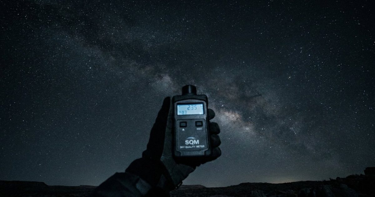
A Sky Quality Meter (SQM) costs $155 to $287 USD and delivers a quantitative zenith sky brightness reading in under three seconds. Unihedron in Grimsby, Ontario, Canada is the only manufacturer. Three main variants serve different purposes: the SQM-L for handheld single readings, the SQM-LU for USB-connected logging, and the SQM-LU-DL for standalone datalogger operation that needs no PC on site. Choosing wrong creates data incompatibilities that invalidate longitudinal comparisons. This guide explains what the instrument actually measures, where each variant belongs, and what it cannot do. For the broader measurement context — satellite data, all-sky cameras, LoNNe calibration — see our overview of light pollution measurement methods.
What an SQM Actually Measures
A silicon photodetector behind a Hoya CM-500 filter samples the zenith sky and returns a single number in mag/arcsec².
The SQM sensor is a TAOS TSL237S light-to-frequency converter paired with a Hoya CM-500 near-infrared cut filter. The filter passes the visible band — approximately 320 to 720 nm — and blocks the infrared. The photodetector converts photon flux into a frequency signal, which the firmware translates into astronomical magnitudes per square arcsecond (mag/arcsec²). Higher numbers mean darker skies. A reading of 22.0 is pristine dark; 20.0 is rural with a visible glow on the horizon; below 18.0 is urban.
The result is a single-pointing zenith measurement. That is the instrument’s strength and its hard boundary. The SQM-L and all lens-equipped variants use a narrow field of view: approximately 10° half-width at half maximum (HWHM), which corresponds to a 20° full-width at half maximum (FWHM) acceptance cone. The original SQM without a lens has a much wider acceptance angle — roughly 42° HWHM — sampling a large portion of the hemisphere. Readings from the original SQM and the SQM-L are not interchangeable. The wider-field model collects more horizon glow, producing systematically lower (apparently brighter) readings at suburban sites where the zenith sky is relatively clean but the horizon is orange.
Output is available in two units: mag/arcsec² for astronomers (logarithmic, higher = darker) and millicandela per square metre (mcd/m²) for lighting engineers (linear, higher = brighter). The SQM reports mag/arcsec² natively. The conversion is non-linear and direction-sensitive — do not average the two. What the SQM does not measure: horizon glow below the acceptance cone, spectral colour of the skyglow, or any part of the hemisphere other than the zenith column.
SQM-L vs. SQM-LU vs. SQM-LU-DL
Same optics across all three variants. The differences are connectivity and data storage — and they determine whether you can run the instrument unattended.
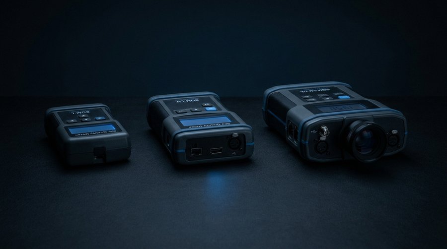
Unihedron’s current lens-equipped product line consists of four models. Prices below are the manufacturer’s USD list price as of 2025 (store.unihedron.com):
| Model | Interface | Display | Datalogger | Price (USD) | Best for |
|---|---|---|---|---|---|
| SQM-L | None (standalone) | LCD | No | $155 | Handheld field readings, hobby observing, workshop tutorials |
| SQM-LU | USB | None | Via PC | $218 | Researcher setups, citizen science networks with PC on site |
| SQM-LU-DL | USB | None | Built-in | $287 | Remote fixed-mount monitoring, no PC required on site |
| SQM-LR | RS232 | None | Via host | — | Weather station integration, industrial serial bus setups |
All lens variants share the same 20° FWHM acceptance cone, the same Hoya CM-500 filter, and the same ±0.10 mag/arcsec² single-unit repeatability. What differs is what happens to the data after the measurement.
The SQM-L shows the reading on its built-in LCD. You read it, write it down, and move on. There is no USB port and no automated logging. For someone doing occasional sky quality checks at an observatory or running a public outreach session, this is sufficient. It is the instrument most LoNNe training schools used for participants’ first-contact measurements.
The SQM-LU has no display. It connects via USB to a laptop or Raspberry Pi, which runs Unihedron’s SQM Reader software or a third-party logging script. The PC handles timestamping, averaging, and file storage. This is the standard choice for citizen science network nodes where a permanent computing board is acceptable — a Pi Zero at a rural monitoring station, for instance. Cross-calibration between SQM-LU units in a network is straightforward because data are timestamped and logged automatically.
The SQM-LU-DL adds onboard flash memory to the LU optical assembly. Plug it in, orient it at the zenith, walk away. It records measurements at configurable intervals and stores them internally. Periodic downloads via USB retrieve the full dataset. LoNNe recommended the LU-DL for unmanned multi-night campaigns because no observer presence is required — an observer’s body heat and breathing create stray thermal gradients and micro-vibration that affect the immediate environment. An unattended unit in a fixed weatherproof mount does not. For cross-calibration protocols specific to network deployments, see our article on the LoNNe intercomparison campaigns.
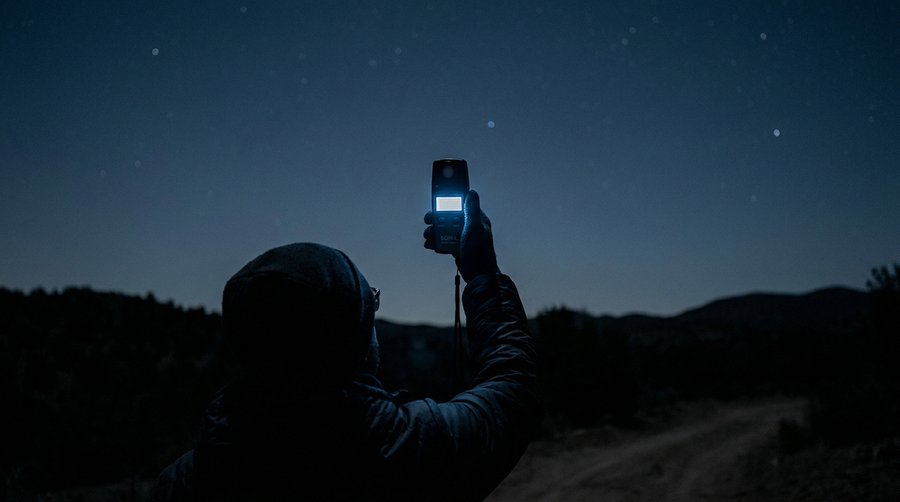
How to Use an SQM Correctly
Point it straight up. Wait three seconds. Repeat three times and use the median. Everything else is protocol noise.
Six rules cover most field errors:
1. Point at zenith. The 20° FWHM cone captures whatever is directly overhead. A five-degree tilt toward a nearby streetlamp shifts the reading by 0.05 to 0.2 mag/arcsec² depending on how bright that source is. Use a spirit level if the instrument is fixed-mounted.
2. Clear the acceptance cone. No trees, roof edges, or structures within the 20° radius around zenith. Rooftop vents in particular reflect scattered light upward at low angles into the cone.
3. Take three readings and use the median. Single readings fluctuate by ±0.05 mag/arcsec² due to atmospheric scintillation and sensor noise. Three readings with the median value eliminates single-shot outliers.
4. Avoid direct light sources. A car headlight or flashlight within ten metres while taking a reading corrupts the result instantly. Dark-adapt your eyes if making manual readings; cover the instrument with your body if unexpected light appears.
5. Temperature compensation is built in, but the instrument needs five minutes to equilibrate to ambient air temperature after coming from indoors. A sensor at 22°C measuring a 5°C night sky gives a reading that drifts by up to 0.1 mag/arcsec² in the first minutes.
6. Below Bortle 8, readings below 18.0 mag/arcsec² are expected. Above Bortle 8 (deep urban), sensor noise begins to approach the signal at very bright readings. The SQM is most reliable at Bortle 3 to 6 — where most research-grade monitoring happens. For context on how Bortle classes map to SQM values, see our guide to measurement methods and units.
Common mistakes that produce bad data: reading through window glass (transmission losses of 6-20% at UV/blue end); condensation on the sensor face in humid conditions; nearby security lighting triggered mid-measurement; and recording altitude above horizon rather than zenith.
The LED Blindspot
The Hoya CM-500 filter peaks around 500 nm. Modern white LED streetlights do significant work below that, in a band the SQM suppresses.
This is not a manufacturing defect. It is a calibration-era mismatch. When Unihedron developed the SQM in the early 2000s, high-pressure sodium (HPS) lamps dominated street lighting. HPS output peaks at 589 nm — comfortably within the CM-500 passband. The instrument was calibrated for a sodium world.
White LED street lights are different in spectral structure. A blue LED pump at 440 to 480 nm excites a broad-spectrum phosphor layer; the resulting output includes a distinct blue peak below 505 nm. The Hoya CM-500 filter suppresses the SQM’s sensitivity at those wavelengths. Practical consequence: as cities replace HPS fixtures with white LEDs, the SQM underreports the change in zenith sky brightness. Hänel et al. (2018, Journal of Quantitative Spectroscopy and Radiative Transfer, 205: 278–290; arXiv:1709.09558) quantified this using calibrated fisheye cameras with separate colour channels, showing that standard SQMs at LED-retrofitted suburban sites can underreport blue-LED skyglow contribution by roughly 0.2 to 0.4 mag/arcsec² compared to a true broadband brightness measurement.
The practical implication is asymmetric. SQM readings remain internally consistent for longitudinal self-calibration: if your monitoring station has used the same SQM-LU-DL for five years, your trend data is valid on its own terms. You can track whether your site is getting brighter or darker. What you cannot do is compare absolute values across different eras or sites without knowing the lamp type: an SQM reading of 20.5 at an HPS-lit suburban site is not the same sky as an SQM reading of 20.5 at an LED-retrofitted suburban site. The LED site is realistically brighter — in the blue band the SQM does not see. For the LoNNe field campaigns that documented this discrepancy at ground level, parallel to what Kyba et al. (2017) found via VIIRS satellite, see our article on LoNNe intercomparison results. The connection between the satellite blindspot and the ground-instrument blindspot is the same LED transition, seen from two different altitudes.
Citizen Science Deployment
A fixed SQM-LU-DL on a north-facing roof, logging nightly, feeding data to Globe at Night’s monitoring network — that is the standard setup for a long-term unattended station.
Globe at Night, operated by NOIRLab, runs annual campaigns based on naked-eye limiting magnitude (NELM) observations. The Globe at Night Sky Brightness Monitoring Network (GaN-MN) extends that with fixed SQM-LE stations — using automatic Ethernet-connected units — that feed a persistent database of nightly readings accessible for download. Individual contributors can submit SQM data via the Globe at Night portal or through national NSBM (Night Sky Brightness Monitoring) networks in their country.
Setting up a citizen monitoring station: mount the SQM-LU-DL in a weatherproof enclosure (PVC pipe cap with optical window is standard) pointing straight up, oriented 90° from any dominant light source if possible. Fix it to a north-facing roof on a structure unlikely to be modified. Configure the logging interval — 60 seconds is standard for research-grade continuity. Schedule nightly automatic downloads with a Raspberry Pi if you want remote access; otherwise do monthly manual USB downloads. Submit data to the Globe at Night Sky Brightness Monitoring Network or your national NSBM coordinator.
Network effects are real. Single-station SQM data is useful for local trend analysis. When 20 or 100 stations in a region operate with cross-calibrated instruments, the aggregate detects regional lighting policy effects that single sites cannot resolve. Falchi et al. (2016, Science Advances) anchored the World Atlas of Artificial Night Sky Brightness with more than 35,000 ground-based SQM measurements — most contributed by non-professional observers. The aggregate is the scientific output. For the policy dimension of what coordinated citizen data has already achieved, see our article on light pollution solutions and regulation. For a step-by-step guide to Globe at Night observation, see our Globe at Night tutorial.
When an SQM Is Not Enough
A single zenith photometer cannot map the hemisphere, separate lamp spectra, or track the blue shift that defines the current LED transition. For those questions, you need different tools.
The next step up is an all-sky photometer. Hänel et al. (2018) benchmarked five instrument classes and concluded that calibrated DSLR cameras with fisheye lenses provide the best ratio of ease-of-use to information richness: a single 180° exposure yields sky brightness across the full hemisphere in three colour channels within five minutes of processing. The blue channel captures LED contribution that the SQM misses. An all-sky camera costs roughly the same as a mid-range DSLR plus a fisheye lens — roughly €400 to €800 for a competent setup — but requires calibration, dark frames, and some astrophotography workflow knowledge.
The TESS-W photometer from the STARS4ALL network (UCM Madrid, H2020 project 688135) is a fixed-mount alternative designed specifically for light pollution monitoring. Priced at €275 (guaix.fis.ucm.es), it connects via WiFi and streams data in real time. The TESS-4C variant adds four spectral channels, giving it sensitivity across the visible band that the standard SQM lacks. TESS-W units feed the STARS4ALL network database. For LED-transition sites where spectral shift matters — any city that has undergone large-scale LED retrofitting since 2015 — TESS-W with multiple channels is a better choice than a standard SQM alone.
For professional-grade spectral decomposition, a spectroradiometer separates sodium and LED contributions wavelength by wavelength. LoNNe intercomparison campaigns deployed spectroradiometers at every site to give the field the spectral ground truth that broadband instruments cannot provide. Cost is typically €3,000 to €15,000 depending on resolution and sensitivity. That budget is out of range for most citizen science setups — but if you want to publish on sodium-to-LED spectral shift at your monitoring site, an SQM alone will not get the paper across a reviewer.
FAQ
Which SQM should I buy for my first measurements?
Start with the SQM-L ($155 USD) if you want handheld readings at different sites, star parties, or outreach events. The LCD display means no laptop needed. If you are setting up a fixed monitoring station and plan to log data over months or years, skip directly to the SQM-LU-DL ($287 USD) — its built-in datalogger removes the dependency on a permanently powered computer and is what LoNNe recommended for unattended campaigns.
Do SQM readings change by season?
Yes, and predictably. Airglow — natural oxygen and sodium emission from the mesosphere — varies with solar activity and season, contributing a background of roughly 22.0 mag/arcsec² at a pristine site. Summer nights are shorter and airglow tends to be slightly elevated in geomagnetically active periods. Seasonal Milky Way position affects the diffuse starlight component detectable at dark sites. Comparing raw readings across seasons without logging date, moon phase, and approximate atmospheric extinction introduces genuine variability that can be mistaken for light pollution trend. Log the metadata, not just the mag/arcsec² value.
Can I measure from my city balcony?
You can take a reading. At Bortle 7 to 9 (typical inner-city or bright suburban), the SQM will return numbers — often 18.0 to 19.5 mag/arcsec². The reading is valid for that zenith column at that moment. What it does not represent: the full hemisphere brightness, the horizon glow that probably dominates your light pollution exposure, or a comparable “site quality” score in the way rural sites are rated. Balcony readings are useful for tracking change at a fixed location over time; they are not comparable to field readings from dark sites without careful context. Surrounding structures and reflective surfaces also complicate the 20° FWHM cone.
How do SQM readings compare internationally?
They do not compare cleanly without cross-calibration. The LoNNe intercomparison campaigns established that two SQM-L units of the same model, measured at the same site on the same night, can disagree by up to ±0.19 mag/arcsec² in field conditions — nearly four times the annual sky-brightness trend from LED deployment. Any database that combines SQM readings from different contributors without explicit cross-calibration carries that uncertainty floor. Globe at Night’s monitoring network requests calibration data alongside station submissions. Use that protocol if your goal is data that can be pooled with international datasets rather than trend analysis at a single site.