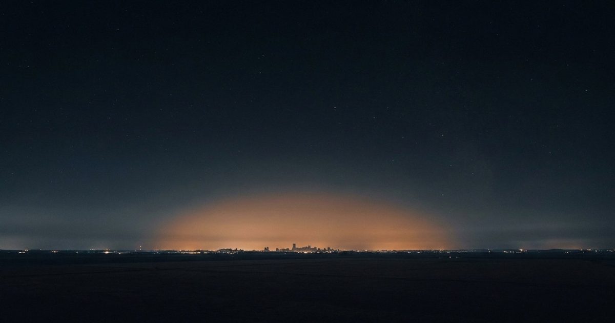
Skyglow is the atmosphere’s answer to artificial light — not the light itself, but the scattered fraction that returns earthward as a diffuse luminous haze. Falchi and Cinzano’s radiative transfer models integrate light contributions out to approximately 195 km from each ground point, which explains why a large city lights up the horizon of dark reserves well beyond its boundary. This article covers the physics, the atmospheric variables that amplify it, how it is measured, and what actually brings the glow down. For the broader context on light pollution types, see light pollution: science, ecology, and solutions.
What Skyglow Is — Physics in Plain Terms
Skyglow is not the light you see from a city — it is the atmospheric response to that light, the scattered fraction that returns earthward as diffuse luminous haze.
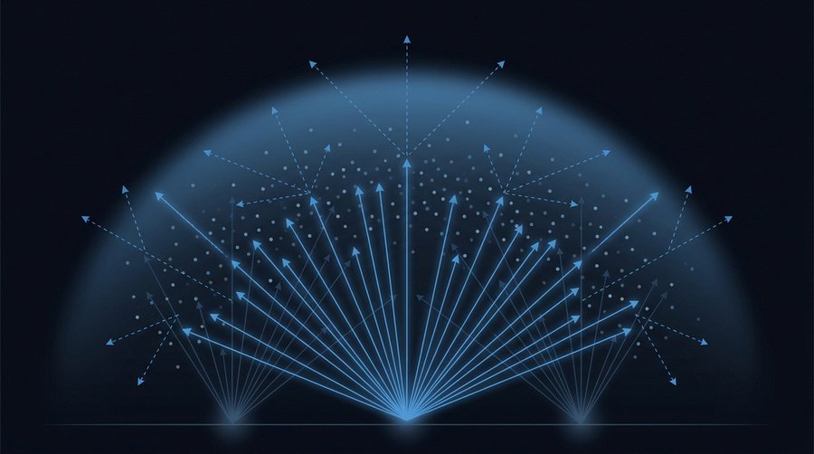
Two scattering mechanisms are at work, and they behave differently enough that conflating them produces bad engineering decisions.
Rayleigh scattering is the interaction of photons with gas molecules — nitrogen, oxygen — whose diameters are far smaller than the wavelength of visible light. The scattering cross-section varies with the inverse fourth power of wavelength. Blue light at 450 nm scatters approximately 5.5 times more efficiently than red light at 700 nm. This is why the daytime sky is blue. It is also why blue-rich LED street lighting at 4,000 K and above contributes disproportionately to skyglow per lumen compared to warm-white alternatives at or below 3,000 K. The physics has been established since Lord Rayleigh in 1871. Its application to street lighting specification is still being ignored in most EU procurement processes.
Mie scattering operates on larger particles: aerosols, dust, fine water droplets. It is not strongly wavelength-dependent — it scatters visible light more uniformly — and it scatters preferentially in the forward direction. In practice, aerosol-laden air captures horizontally propagating photons and redirects them toward the zenith, extending the reach of a city’s light dome well beyond what Rayleigh physics alone would predict. Cities embedded in industrial haze — the Po Valley, the Rhine-Ruhr conurbation — produce skyglow domes that are broader and brighter than comparably sized cities in clean mountain air.
Skyglow is cumulative. Every unshielded luminaire within a region contributes to a shared atmospheric scattering field. No single fixture is individually responsible. The glow is the sum — which is why it resists local fixes and depends on coordinated regional policy.
Why Skyglow Reaches So Far
Walker’s Law gives the quantitative answer: skyglow brightness scales as city population times distance to the power of negative 2.5 — steeper than simple geometry, because the atmosphere adds its own attenuation on top of geometric spreading.
In 1977, Merle F. Walker of Lick Observatory measured sky brightness at varying distances from several Californian cities, publishing the results in the Publications of the Astronomical Society of the Pacific (89: 405–409). The empirical relationship: b = C × P × d^(-2.5), where b is sky brightness in nanoLamberts, P is city population, d is distance, and C is an empirical constant. That formula is built into the Falchi et al. 2016 radiative transfer models.
The exponent of negative 2.5 is not arbitrary. An inverse-square law — pure geometry — gives negative 2.0. The extra steepening reflects atmospheric absorption and forward scattering along the path: photons from near-horizon sources traverse a longer atmospheric column and lose intensity faster than geometry alone predicts. Doubling the distance from a city reduces skyglow by a factor of approximately 5.7, not 4. Cities are large distributed sources rather than point sources, so the cumulative footprint is far wider than a single-emitter calculation would suggest.
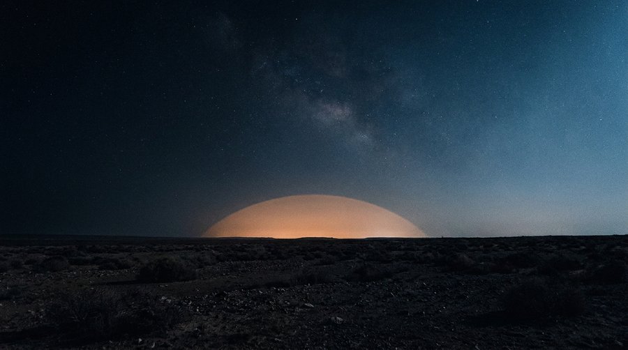
Walker’s Law holds to about 50–100 km. At greater distances, terrain masking and Earth’s curvature cause faster falloff than the model predicts. Falchi and Cinzano integrate contributions out to ~195 km — acknowledging that skyglow influence, while diminishing steeply, is non-zero at that distance under clear conditions.
Three European examples: Berlin’s light dome is visible from Westhavelland Nature Park, 70 km west, which achieves SQM readings of 21.6–22.0 mag/arcsec² despite proximity to a city of 3.7 million. Madrid’s skyglow extends into the Sierra de Guadarrama at distances exceeding 60 km. Milan and the Po Valley conurbation are identifiable from Swiss Alpine sites at 2,000 m elevation and 100 km distance under clear winter conditions. These are not exceptional events. They are the standard reality of light pollution geography in a densely settled continent. For the measurement context, see measuring light pollution: methods, data, and research tools.
What the Atmosphere Does to It
The atmosphere is not a passive medium for skyglow — it is an amplifier whose gain shifts with aerosol load, humidity, cloud cover, and ground-surface albedo.
Aerosol optical depth (AOD) quantifies aerosol-induced scattering in a vertical atmospheric column. High AOD — typical of urban air, industrial corridors, coastal fog — increases forward Mie scattering and raises zenith sky brightness. Falchi and Cinzano used a horizontal visibility of 26 km in their standard model; real-world visibility in the Rhine-Ruhr or Po Valley during winter inversions is often worse, meaning their maps underestimate skyglow in exactly those hotspot regions.
Clouds are the most dramatic variable. An overcast layer acts as a retroreflector: upward light hits the cloud base, scatters back down, re-illuminates ground infrastructure, and returns skyward in a feedback loop. Jechow and Hölker, publishing in the Journal of Imaging in 2019, quantified this at a suburban site near Berlin: zenith luminance amplification factors of up to 188 for snow-and-cloud combined, and 33 for snow alone on a clear night. They called the effect snowglow. From Stockholm’s perspective this is routine — winter inversions and snowpack together turn the southward horizon into a diffuse white wall that holds through the night.
Volcanic aerosols provide a rare historical calibration point. Following the 1991 eruption of Mount Pinatubo, stratospheric AOD increased by a factor of 10 to 100 above pre-eruption levels. The sulfuric acid aerosol cloud spread globally within weeks and persisted for more than two years. The underlying physics is clear: any increase in stratospheric aerosol load increases forward scattering of upward-directed artificial light, raising both the intensity and angular spread of skyglow. Pinatubo was, for two years, a global amplifier of every city’s light dome.
How Skyglow Is Measured
Three instrument classes each capture a different slice of the same phenomenon — and each has a blind spot the others partially correct.
The Sky Quality Meter (SQM) is the field standard for point measurements. A silicon photodetector behind a narrowband filter near 550 nm reports zenith sky brightness in mag/arcsec² in under three seconds. The SQM-L — narrow field, ~20° FWHM — is what LoNNe intercomparison campaigns standardised on for research-grade work, costing around EUR 100–150. For variant comparisons and purchasing guidance, see our SQM buyer’s guide: L vs. LU vs. LU-DL.
The SQM’s skyglow limitation: it reads only the zenith. Skyglow often peaks at low elevation angles toward the city, where forward Mie scattering concentrates the dome. A moderate zenith reading can coexist with a dramatically brighter low-elevation hemisphere. All-sky cameras with calibrated fisheye lenses solve this — a single 180° exposure captures the full hemisphere in three colour channels, resolving dome structure, source direction, and angular extent. Hänel et al. (2018, Journal of Quantitative Spectroscopy and Radiative Transfer, 205: 278–290; arXiv:1709.09558) demonstrated that calibrated consumer fisheye cameras provide the best balance of ease and information richness of any instrument class tested. This conclusion shaped LoNNe’s recommendation to adopt all-sky photometry as the intercomparison gold standard.
VIIRS DNB — the Day/Night Band aboard Suomi-NPP and NOAA-20 — provides global coverage but carries a critical spectral limitation: its window runs from 505 to 890 nm. Modern white LED street lighting emits a significant fraction of its energy in the 380–505 nm blue band, below that threshold. VIIRS cannot see the blue light that LED retrofits are adding to the sky. As cities replace sodium lamps with LEDs, satellite data systematically underreports the change. The same LED blindspot that affects SQM calibration documented by Hänel et al. 2018 applies at orbital altitude. For the full spectral gap analysis, see the VIIRS section in measuring light pollution.
Skyglow in Europe — Regional Variations
Europe’s skyglow geography concentrates in specific industrial corridors — and it is not improving in most of them.
Falchi et al. (2016, Science Advances), calibrated against more than 35,000 SQM ground observations, produced the definitive European map. The Po Valley, BeNeLux coastal plain, and Rhine-Ruhr conurbation form a near-continuous maximum-intensity band from the Adriatic to the North Sea. Bortle Class 1 — natural darkness, SQM above 21.7 mag/arcsec² — is inaccessible within hundreds of kilometres of these zones.
The refugia that survive are instructive. Galloway Forest Park in southwest Scotland — 78,000 ha, Europe’s first IDA Dark Sky Park (November 2009) — reaches peak SQM readings of 23.6 mag/arcsec² in its dark-core interior, shielded by the Galloway Hills and the Irish Sea from Scottish urban glow. Westhavelland Nature Park in Brandenburg — 75,000 ha, Germany’s first Dark Sky Reserve (2014) — achieves 21.6–22.0 mag/arcsec² despite sitting 70 km from central Berlin, a consequence of flat wetland topography and the capital’s east-facing emission geometry. Øvre Pasvik National Park in Finnmark, Norway — 11,900 ha, designated July 2024 — reaches Bortle Class 1–2 at 69°N during polar night. Full profiles at dark sky places in Europe, Galloway Forest Park, and Westhavelland.
France offers the only documented national improvement. The Arrêté of 27 December 2018 — the only EU national law specifying both a CCT ceiling (3,000 K) and an upward light ratio cap (ULR ≤1%) — has produced measurable results. ANPCEN’s Villes et Villages Étoilés programme: certified communes use ~33% less outdoor lighting than the French national average. France’s statistics office (SDES) reports a 19% reduction in high-level light pollution exposure across mainland France between 2014 and 2023. No other EU member state has equivalent documented national data. See France’s 2018 lighting decree for the full policy anatomy.
What Reducing Skyglow Actually Requires
Skyglow reduction requires three simultaneous constraints — upward flux, spectrum, and aggregate output — not one.
Full cutoff fixtures rated BUG U0 under IES TM-15 — zero upward light in nominal installation — are the structural baseline. Any fraction of flux above the horizontal enters the Rayleigh and Mie scattering field regardless of fixture efficiency. France’s ULR cap of 1% is the only national numerical upward light ratio limit in EU law, and a weaker-but-enforceable proxy for BUG U0 performance at national scale.
CCT at or below 3,000 K is the spectral constraint. Because Rayleigh scattering scales with the inverse fourth power of wavelength, a blue-rich source at 4,000 K contributes substantially more skyglow per lumen than a warm-white source at 2,700 K of identical photopic output. EN 13201 — Europe’s primary road-lighting standard — specifies no CCT requirement. An M1-class installation at 6,500 K is fully compliant with EU road-lighting law while maximising skyglow contribution. LoNNe explicitly recommended incorporating spectral requirements into EN 13201. The recommendation was not adopted.
The third constraint is aggregate output. Kyba et al. (2017, Science Advances) found Earth’s lit surface growing at 2.2% per year during 2012–2016 — the peak of the LED transition. Kyba et al. (2023, Science 379: 265–268), using Globe at Night citizen data from 51,351 observers, found sky brightness growing at 9.6% per year between 2011 and 2022. The gap between those two figures — 2.2% satellite, 9.6% ground-based — is the LED blindspot quantified. Both numbers say the same thing: efficient fixtures deployed in greater numbers and at higher lumen packages produce more skyglow. The Jevons mechanism is the central dynamic. Efficient fixtures without output caps accelerate the problem. For the evidence on LED rebound, see the LED paradox and Jevons effect.
For the full context of ALAN beyond skyglow, see ALAN: the research framework. For the satellite constellation dimension — a new unregulated contributor to skyglow — see satellite constellations and light pollution.
Frequently Asked Questions
How far can skyglow from a single city reach?
Walker’s Law (Walker 1977, PASP 89:405–409) predicts skyglow scales as population times distance to the power of negative 2.5, holding to about 50–100 km from a city. Falchi and Cinzano’s radiative transfer models integrate light contributions out to approximately 195 km under standard atmospheric conditions. For the largest metropolitan areas, measurable sky-brightness influence can extend well beyond 100 km on clear winter nights. 200 km is a physically justified upper bound for light-dome influence, not the typical strong-skyglow radius.
Why is blue light worse for skyglow?
Rayleigh scattering cross-section scales with the inverse fourth power of wavelength: blue light at 450 nm scatters approximately 5.5 times more efficiently than red light at 700 nm. White LED street lighting at 4,000 K and above emits disproportionately more blue-spectrum power than warm-white equivalents at or below 3,000 K. A blue-rich source therefore contributes more skyglow per delivered lumen than a warm source of identical photopic output. Reducing CCT to 3,000 K or below is the fastest spectral fix available — and still unrequired by EN 13201.
Can skyglow be reduced without turning off lights?
Yes. Full cutoff fixtures (BUG U0 — zero upward flux), CCT at or below 3,000 K, and adaptive dimming after midnight each reduce skyglow without eliminating service. France’s 2018 decree combines all three with curfews for non-essential categories, achieving a 19% reduction in high-level light pollution exposure across France between 2014 and 2023. The constraint that makes it work: output caps must accompany efficiency improvements, or the Jevons mechanism erases the gain.
Is skyglow the same as light pollution?
Skyglow is one of five recognised forms of light pollution — the most spatially extensive. It results from atmospheric scattering of upward-directed artificial light, not from direct surface illumination. Unlike glare or light trespass, it is cumulative and regional: every unshielded luminaire contributes to a shared atmospheric field, which is why fixing it requires coordinated policy, not just individual fixture changes. For the full five-form taxonomy, see light pollution: science, ecology, and solutions.